The professional’s guide to Quantum Technology
- Preface: Why this guide?
- Part 1 – The background: Why are we so enthusiastic about Quantum Technology?
- Part 2 – The applications: What problems will we solve with Quantum Computers?
- Part 3 – The developments: Searching for a killer application, with a closer look at artificial fertilizer
- Part 4 – The applications of Quantum Networks
- Part 5 – Timelines: When can we expect a useful quantum computer?
- Part 6 – Getting started: What steps should your organization take?
- Part 7 – The hardware: Why you should care about different qubits
- Part 8 – The threat: The impact on cybersecurity
- Part 9 – Scaling up: Why we need error correction
- Further reading: An overview of resources
Part 9 – Why we need error correction
At a glance:
- To run long computations, we need to dramatically reduce the likelihood of error of each elementary step – not just a little bit, but by a factor of millions.
- Error correction is the most effective method to achieve extremely low error probabilities. It combines a small number of ‘physical’ qubits (think of several hundreds) into a single ‘logical’ qubit that suppresses errors exponentially.
- Logical qubits are still not perfect qubits: the ‘number of steps’ that they can survive is an important specification that determines whether they can run your application.
The recently announced roadmap by QuEra caused quite a buzz: the startup presents its plans in terms of logical qubits, aiming to have 100 of these by 2026. This is a significant shift from their earlier focus on physical qubits. Experts agree that achieving error correction is one of the key milestones towards large-scale computations, like breaking cryptography. As we expect many breakthroughs in error correction in the years to come, this is the right time to understand the importance of error correction and clear up some misconceptions about logical qubits.
A statement that we often hear is the following (which is incorrect!)
"Logical qubits (or: error-corrected qubits) are resilient to errors that occur during a computation. Once we have logical qubits, we can increase the length of our computations indefinitely. "
What’s the problem here? Well, not every logical qubit is created equally. We expect to soon see logical qubits that are perhaps 2x more accurate than today’s bare hardware qubits, and later 10x, and in the future perhaps 1000x. Error correction is a trick to reduce the probability of errors, but it will not eliminate errors completely. In the following decade, we expect to see gradual improvements, hopefully down to error rates of 10-10 and below. Let’s explore the reasons behind this.
What is error correction?
In quantum error correction, we combine some number (think of hundreds or thousands) of ‘physical’ hardware qubits into a virtual ‘logical’ qubit. The logical qubits are the information carriers used in an algorithm or application. Error correction methods can detect whenever tiny errors occur in the logical qubit, which can then be ‘repaired’ with straightforward operations. Under the assumption that the probability of hardware errors is sufficiently low (below a certain error threshold), the overall accuracy improves exponentially when we combine more physical qubits per logical qubit. Hence, we obtain a very favourable trade-off between the number of qubits, and the accuracy of the qubits.

Doesn’t measuring a quantum state destroy the information in the qubits?
Indeed, if we naively measure all the physical qubits, then that would destroy the computation. However, quantum error correction uses an ingenious way to measure only whether or not an error occurred. It learns nothing about the actual information content of the qubit. It turns out that this way, the data stored in the logical qubit is not affected.
Why are errors so much of a problem? How do errors screw up our computations?
In short: even tiny errors are a problem because we want to perform incredible numbers of quantum operations — think of billions or trillions of them.
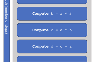
Let’s make this more concrete. A computer program is essentially a sequence of ‘steps’, each of which a computer knows how to perform. We say that a program or algorithm has a width, which is the number of qubits it requires. It also has a depth, which is the number of consecutive steps that need to be performed. In early hardware, you may interpret one step as a single quantum gate.

Let’s look at a very simple model of a computer, which is not unlike what happens inside a quantum computer or a modern (classical) CPU. As above, the computer is supposed to work through a list of instructions. We can consider various specifications of a computer:
- The available memory, measured in bits (or perhaps megabytes or gigabytes, if you like).
- The speed at which the computer operates, measured in steps per second.
- The “probability of error”, the chance for each computational step to introduce some mistake. This is given as a number between 0 and 1 (or a percentage between 0 and 100%). Many sources use the word ‘fidelity’ instead, which can be roughly interpreted as the opposite (fidelity ≈ 1 – probability of error). In this text, we sometimes just say “error”.
In this simple model, the time taken to complete the computation equals: “depth” x “speed”. You can make a computer program faster by increasing the speed of the computer, or by writing a ‘better’ program that takes fewer steps.
The influence of errors is harder to track. For contemporary computers, we typically don’t worry about hardware mistakes at all: every step has essentially 100% certainty to output the correct result. Unfortunately, in our little model, this is not the case.
Assume that each step has a 1% (= 10-2) chance of error. What will the impact on the final computation be? Here, we compute the chance to finish the computation without any errors, for various numbers of total steps:
| Error probability: 1% | |
| Number of steps | P(success) |
| 1 | ( 0.99 )1 = 99% |
| 100 | ( 0.99 )100 = 37% |
| 1000 | ( 0.99 )1000 = 0.004 % |
| 10,000 | ( 0.99 )10,000 = 10-44 |
In this simple model, we assume that any error is catastrophic. This is quite accurate for most programs. You might argue that there is a miniscule chance that two errors cancel, or that the error has very little effect on the final result, but it turns out that such effects are statistically irrelevant in large computations.
Now, assume we improve our hardware, towards an error rate of 0.1% (=10-3), then we find:
| Error probability: 0.1% | |
| Number of steps | P(success) |
| 1 | ( 0.999 )1 = 99.9% |
| 100 | ( 0.999 )10 = 90% |
| 1000 | ( 0.999 )1000 = 37% |
| 10,000 | ( 0.999 )10,000 = 0.004 |
A probability to succeed of 37% sounds bad, but for truly high-end computations we might actually be okay with that. If the program results in a recipe for a brand-new medicine, or if it would tell us the perfect design for an aeroplane wing, then surely we don’t mind repeating the computation 10 or 100 times, after which we’re very likely to learn this breakthrough result. On the other hand, if the probability of success is 10-44, then we will never find the right result, even if the computer repeats the program billions of times.
In the table above, we see a pattern: to reasonably perform 102 steps, we require errors of roughly 10-2 or better. To perform 103 steps, we need roughly a 10-3 chance of error. These are very rough order-of-magnitude estimates, but they have a very useful conclusion when dealing with very large circuits (or very small errors): if you want to execute 10n steps, you’d better make sure that your error probability is not much bigger than 10-n.
This simplified model assumes that an operation either works correctly, or it fails, but nothing in between. In reality, quantum operations act on continuous parameters, and therefore they have an inherent, scalar-value accuracy. For example: a quantum gate might change a parameter from A to A+0.49, where it’s supposed to do A+0.5. For our discussion, this doesn’t really matter — for our qualitative conclusions, it suffices to see a “99% accurate” quantum gate as simply having a 99% chance of succeeding. We also overlook various other technical details, operations carried out in parallel, different types of errors, native gate sets, connectivity, and so forth — these make the story much more complicated, but will not change our qualitative conclusions.
Longer computations => more qubits
As problems become ‘more complex’, they typically require more from our computers: both in terms of width (number of bits) and depth (number of steps). We could illustrate this as below. You can think of a number “N” as the difficulty or the size of the problem: for example, we might consider the problem of “factoring a number that can be written down using at most N bits”).

Keep in mind: we’re talking about the requirements to solve a problem here, so that width indicates logical bits. If a computer does not have error correction, then 1 logical bit is simply the same as 1 physical bit – or its quantum equivalent.
For ‘perfect’ classical computers, the situation is straightforward: if a problem gets bigger, then we need more memory, and we need to wait longer before we obtain the result. For (quantum) computers that make errors, the situation is more complex. With increasing depth, not only do we need to wait longer, we also need to lower the error probabilities, and hence, need more advanced error correction.
Let’s consider two computers for which we show the width and depth that they can handle (where the available ‘depth’ is essentially 1 / probability of error). On the left is a computer without error correction (hence it has a small, fixed depth). The other is an error-corrected computer that can trade between depth and width (in certain discrete steps).

The computer without error correction might have enough memory to solve a problem, but often lacks the depth. Even an error-corrected computer might not have a suitable trade-off to solve the hardest problems. Looking at the above example, it seems that both computers can solve the N=10 problem. Here, only the error-corrected computer can solve the N=20 problem, as depicted below. For the N=40 problem, the error-corrected computer might have sufficient depth OR sufficient width, but it doesn’t have both at the same time. Hence, neither computer solves the N=40 problem.

Towards cracking the N=40 problem, our best bet is to upgrade the error-corrected computer to have more physical qubits. Using error-correction, these can then be traded to achieve sufficient depth (whilst also reserving just enough logical qubits to run the algorithm).
We have found an interesting conclusion here. Larger problems not only require more memory (to store the calculation), but also more depth, which requires more qubits again! To summarise:
‘Harder’ problems -> More depth -> Better error correction -> More physical qubits
Effectively, once we reach an era of error correction, then increasing the number of physical qubits will still be among the top of our wishlist.
Further reading:
- Craig Gidney (Google) has a more technical blog post on why adding physical qubits will remain relevant in the following decades.
- [Technical!] Some scientific work speaks of ‘early fault-tolerant’ quantum computing, such as:
- “Early Fault-Tolerant Quantum Computing”, discussing how we can squeeze as much as possible out of limited devices.
- “Assessing the Benefits and Risks of Quantum Computers” takes a similar width x depth approach as we do here, but uses it to assess what applications will be within reach first.
[Technical] What is the current state-of-the-art?
As of January 2024, there have been several demonstrations of error correction (and the slightly less demanding cousin: error detection), but these have all been with limited numbers of qubits, and with very limited benefit to depth (if any at all). However, we seem to be at a stage where hardware is sufficiently mature that we can start exploring early error correction.
Below are the three most popular approaches to error correction. Each of them can be considered a ‘family’ of different methods, based on similar ideas:
- Surface codes
- Color codes
- Low-Density Parity Check (LPDC) codes
The surface code (or toric code) has received a lot of scientific attention, as this seems to be on the roadmap of large tech companies like Google and IBM. Their superconducting qubits cannot interact with each other over long distances, and the surface code can deal with this limitation. Many estimates that we use in this Guide (such as the resources required to break RSA or to simulate FeMoco) are based on this code. It has already been tested experimentally on relatively small systems:
- A team from Hefei/Shanghai experiments with a 17-qubit surface code.
- Google sees improvements when scaling the surface code from 17 to 49 qubits.
Color codes are somewhat similar to surface code, but typically lack the property that only neighbouring qubits have to interact. This makes them less interesting for superconducting or spin qubits, but still they appear to work extremely well for trapped ions and ultracold atoms.
- Startup QuEra demonstrates 48 logical qubits using a color code [Scientific presentation]
- Already in 2014, an early experiment on a single logical qubit (color code) was performed in Innsbruck.
LDPC codes are now rapidly gaining attention. They build on a large body of classical knowledge, and could have (theoretically) more favourable scaling properties over the surface code.
- French startup Alice & Bob are aiming for a unique combination of ‘cat qubits’ together with LDPC codes, which can theoretically match very elegantly.
Which code will eventually become the standard (if any), is still completely open.
See also:
- The Quantum Threat Timeline Report asked several experts what they find the most likely approach to fault tolerance (section 4.5).
What are the main challenges?
Firstly, we would need just slightly more accurate hardware. We mentioned a certain accuracy threshold earlier: state of the art hardware seems to be close to this threshold, but not comfortably over it. Secondly, error correction also requires significant classical computing power, which needs to solve a fairly complex ‘decoding’ problem within extremely small time bounds (within just a few clock cycles of a modern CPU). Classical decoding needs to become more mature, both at the hardware and the software level. It is not unlikely that purpose-built hardware will need to be developed, which for some platforms might be placed inside a cryogenic environment (placing stringent bounds on heat dissipation). Theoretical breakthroughs can still reduce the requirements on classical processing.
Lastly, it turns out that ‘mid-circuit measurements’ are technically challenging: most experiments so far relied on destructively measuring all qubits at the end of an experiment. Without intermediate measurements, one might retroactively detect errors, but one cannot repair them. We should also warn that many related terms such as “error mitigation” and “error suppression” exist. They might be useful for incremental fidelity improvements, but they don’t facilitate an exponential increase in depth like proper error correction does.
See also:
British startup Riverlane builts a hardware chip that ‘decodes’ which error occurred on logical qubits. (Technical report).
Conclusion
The bottom line is that one shouldn’t blindly take ‘logical qubits’ as perfect building blocks that will run indefinitely. A logical qubit is no guarantee that a computer has any capabilities, it merely indicates that some kind of error correction is applied (and it doesn’t say anything about whether this error correction works well at all). A much more interesting metric is the probability of error in a single step (in jargon: the fidelity of an operation), which gives a reasonable indication of the number of steps that a device can handle!